Layout and simulation of a ring resonator with grating couplers¶

Build a small ring circuit with grating couplers. Export the layout + run a circuit simulation to verify circuit operation.

Importing the technology file¶

We start with importing the silicon_photonics technology, which is a basic technology shipped with IPKISS. You can replace this technology by another technology (custom made, or from our list of supported PDKs). and the layers will automatically adjust to reflect this technology.

from technologies import silicon_photonics
from ipkiss3 import all as i3

# Import other python libraries.
import numpy as np
import pylab as plt

Creating the ring resonator¶

Here we use a ring resonator from the picazzo component library (the Picazzo Library is a generic component library with a wide range of photonic components).

from picazzo3.filters.ring import RingRect180DropFilter
my_ring = RingRect180DropFilter()

# Setting the layout properties of the ring.
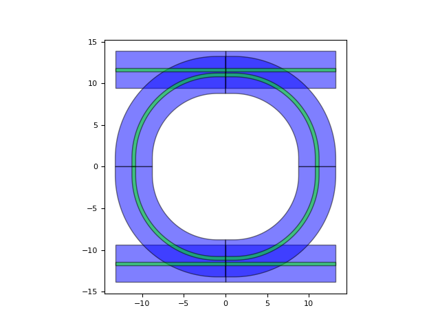
my_ring_layout = my_ring.Layout(bend_radius=10.0)  # We set the bend radius of the ring to 10.
my_ring_layout.visualize()  # We visualize the layout of the ring

<Figure size 640x480 with 1 Axes>

Running a circuit simulation¶

Here we set some simple model parameters for the directional coupler of the ring, and then we run a circuit simulation. Note that the waveguide lengths are automatically extracted from the layout.

cp = dict(cross_coupling1=1j*0.3**0.5,
          straight_coupling1=0.7**0.5)  # The coupling from bus to ring and back

my_ring_cm = my_ring.CircuitModel(coupler_parameters=[cp, cp])  # 2 couplers

# Simulating the ring.
wavelengths = np.linspace(1.50, 1.6, 2001)
S = my_ring_cm.get_smatrix(wavelengths=wavelengths)

plt.figure()
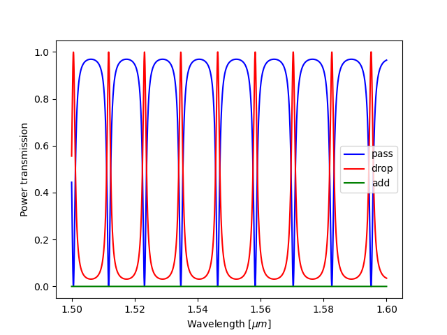
plt.plot(wavelengths, np.abs(S['in1', 'out1'])**2, 'b', label="pass")
plt.plot(wavelengths, np.abs(S['in1', 'out2'])**2, 'r', label="drop")
plt.plot(wavelengths, np.abs(S['in1', 'in2'])**2, 'g', label="add")

plt.xlabel(r"Wavelength [$\mu m$]")
plt.ylabel("Power transmission")
plt.legend()
plt.show()

Creating the grating coupler¶

The picazzo component library also contains parametrized curved grating couplers. We will pick one to use in our circuit.

from picazzo3.fibcoup.curved import FiberCouplerCurvedGrating
my_grating = FiberCouplerCurvedGrating()

# Setting the layout properties of the grating layout.
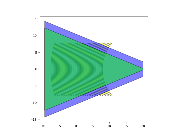
my_grating_layout = my_grating.Layout(n_o_lines=24, period_x=0.65, box_width=15.5)
my_grating_layout.visualize()

# Setting the properties of the circuit model and simulate.
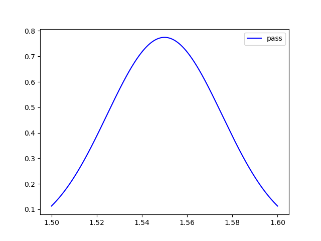
my_grating_cm = my_grating.CircuitModel(center_wavelength=1.55,
                                        bandwidth_3dB=0.06,
                                        peak_transmission=0.60**0.5,
                                        reflection=0.05**0.5)

S = my_grating_cm.get_smatrix(wavelengths=wavelengths)
plt.figure()
plt.plot(wavelengths, np.abs(S['vertical_in', 'out'])**2, 'b', label="pass")
plt.legend()
plt.show()

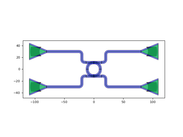
Creating a small circuit with the ring and grating coupler¶

Next, we can use some high-level routing functionality from IPKISS to place the grating couplers and the ring, and route waveguides between them. This is done using ipkiss3.all.Circuit.

distance_x = 100.0
distance_y = 30.0

my_circuit = i3.Circuit(
    insts={
        'in_grating': my_grating,
        'pass_grating': my_grating,
        'add_grating': my_grating,
        'drop_grating': my_grating,
        'ring': my_ring
    },
    specs=[
        i3.Place('ring', (0, 0)),
        i3.Place('in_grating', (-distance_x, -distance_y)),
        i3.Place('pass_grating', (distance_x, -distance_y), angle=180),
        i3.Place('add_grating', (distance_x, distance_y), angle=180),
        i3.Place('drop_grating', (-distance_x, distance_y)),
        i3.ConnectManhattan([
            ("in_grating:out", "ring:in1"),
            ("pass_grating:out", "ring:out1"),
            ("add_grating:out", "ring:in2"),
            ("drop_grating:out", "ring:out2"),
        ])
    ],
    exposed_ports={
        'add_grating:vertical_in': 'add',
        'drop_grating:vertical_in': 'drop',
        'in_grating:vertical_in': 'in',
        'pass_grating:vertical_in': 'pass'
    }
)

my_circuit_layout = my_circuit.Layout()

my_circuit_layout.visualize()

# Simulate the circuit.
my_circuit_cm = my_circuit.CircuitModel()
S = my_circuit_cm.get_smatrix(wavelengths=wavelengths)


plt.figure()
plt.plot(wavelengths, np.abs(S['in', 'pass'])**2, 'b', label="pass")
plt.plot(wavelengths, np.abs(S['in', 'drop'])**2, 'r', label="drop")
plt.plot(wavelengths, np.abs(S['in', 'add'])**2, 'g', label="add")
plt.plot(wavelengths, np.abs(S['in', 'in'])**2, 'k', label="reflection")
plt.legend()
plt.show()

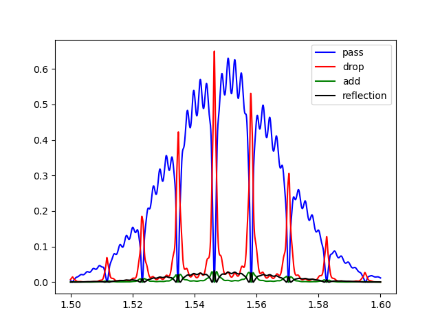
You can clearly see the following features in this response:

the grating response: the grating was designed for 1550 nm, and has a gaussian-like profile,
the ring resonances
there are some ripples on the circuit response, this is due to reflections on the grating couplers.

Caphe is a bidirectional-aware circuit solver (each optical port has a forward and backward propagating wave), and this is how we can capture these important parasitic effects.