WG2

class ipkiss3.cml.WG2(**kwargs)

Single mode polynomial waveguide model.

Uses a polynomial expression of the effective index and loss (in dB/m) as function of wavelength offset.

Parameters

n_eff: List[float]

Polynomial coefficients of the mode effective index as function of wavelength offset from center_wavelength [/m^n]. Highest order first (effective index at center_wavelength last).

loss: List[float]

Polynomial coefficients of the loss of the waveguide mode as function of wavelength offset from center_wavelength [dB/m / m^n]. Highest order first (loss at center_wavelength last).

center_wavelength: float (m)

Center wavelength (in meter) of the model around which n_eff and loss are defined.

length: float (m)

Total length of the waveguide in meter.

Notes

The effective index and loss are calculated as:

\[ \begin{align}\begin{aligned}n_{eff}(\lambda) = n_{eff}[n] + (\lambda-\lambda_c) * n_{eff}[n-1] + ... + (\lambda-\lambda_c)^2 * n_{eff}[0]\\loss(\lambda) = loss[n] + (\lambda-\lambda_c) * loss[n-1] + ... + (\lambda-\lambda_c)^2 * loss[0]\end{aligned}\end{align} \]

Where n is the order of the polynomial, \(\lambda_c\) is the central wavelength at which \(n_{eff}(\lambda_c) == n_{eff}[n]\) and \($loss(\lambda_c) = loss[n]\).

The scatter matrix is given by:

\[\begin{split}\mathbf{S}_{wg}=\begin{bmatrix} 0 & \exp(-j\frac{2 \pi}{\lambda}L n_{eff}(\lambda)) * A \\ \exp(-j\frac{2 \pi}{\lambda}L n_{eff}(\lambda)) * A & 0 \end{bmatrix}\end{split}\]

Where the amplitude loss is calculated as:

\[A = 10^{-loss * L * 1e-4 / 20.0}\]

Terms

Term Name	Type	#modes
in	Optical	1
out	Optical	1

Examples

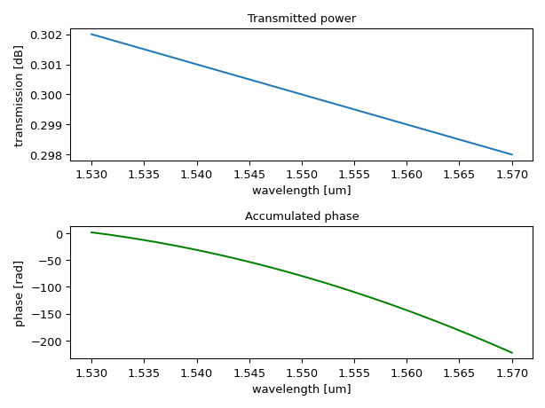
import numpy as np
import ipkiss3.all as i3
import matplotlib.pyplot as plt

# test model
model = i3.cml.WG2(
    n_eff=[-20.0, -0.1, 2.0],
    loss=[1.0 * 100.0, -3.0 * 100.0],
    center_wavelength=1.55e-6,
    length=1000.0 * 1e-6,
)

wavelengths = np.linspace(1.53, 1.57, 2001)
S = i3.circuit_sim.test_circuitmodel(model, wavelengths)

# plot loss and phase
transmission = 10 * np.log10(np.abs(S["out", "in"]) ** 2)
phase = np.unwrap(np.angle(S["out", "in"]))

plt.subplot(211)
plt.plot(wavelengths, transmission)
plt.xlabel("wavelength [um]")
plt.ylabel("transmission [dB]")
plt.title("Transmitted power")
plt.subplot(212)
plt.plot(wavelengths, phase, "g-")
plt.xlabel("wavelength [um]")
plt.ylabel("phase [rad]")
plt.title("Accumulated phase")
plt.tight_layout()
plt.show()

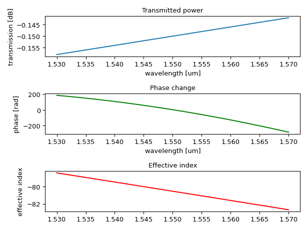
import numpy as np
import ipkiss3.all as i3
import matplotlib.pyplot as plt

# waveguide data
effective_index = 2.4
group_index = 4.5
# use a high GVD to simulate a long waveguide while avoiding large phase jumps
group_velocity_dispersion = 580 * 300 * 1e-12 / (1e-9 * 1e3)  # s /(m * m)
center_wavelength = 1.55e-6  # m
c = 299792458.0  # m /s
length = 1000.0 * 1e-6  # m

# model parameters
dneff_dlambda = (effective_index - group_index) / center_wavelength * 1e-6  # /m
dneff2_dlambda2 = -group_velocity_dispersion * c / center_wavelength * 1e-12  # [/m^2]

n_eff_coefficients = [dneff2_dlambda2, dneff_dlambda, effective_index]
loss_coefficients = [-4.0 * 100.0, 1.5 * 100.0]

# test model
model = i3.cml.WG2(
    n_eff=n_eff_coefficients,
    loss=loss_coefficients,
    center_wavelength=center_wavelength,
    length=length,
)

wavelengths = np.linspace(1.53, 1.57, 2001)
S = i3.circuit_sim.test_circuitmodel(model, wavelengths)

# plot loss, phase and effective index
transmission = 10 * np.log10(np.abs(S["out", "in"]) ** 2)
# unwrap the phase relative to the center wavelength
center_index = np.where(wavelengths == 1.55)[0][0]
phase = np.angle(S["out", "in"])
unwrapped_phase = np.concatenate(
    (np.unwrap(phase[0:center_index][::-1])[::-1], np.unwrap(phase[center_index:]))
)
# calculate neff ourselves - wavelength relative to center_wavelength
neff = np.polyval(n_eff_coefficients, wavelengths - center_wavelength)
plt.subplot(311)
plt.plot(wavelengths, transmission)
plt.xlabel("wavelength [um]")
plt.ylabel("transmission [dB]")
plt.title("Transmitted power")
plt.subplot(312)
plt.plot(wavelengths, unwrapped_phase, "g-")
plt.xlabel("wavelength [um]")
plt.ylabel("phase [rad]")
plt.title("Phase change")
plt.subplot(313)
plt.plot(wavelengths, neff, "r-")
plt.ylabel("effective index")
plt.title("Effective index")
plt.tight_layout()
plt.show()