Building an Aperture
In this tutorial we’ll explore how to build an aperture, which can serve as a building block in the design of a star coupler. As this is one of the steps towards building an AWG you’ll need a valid license to execute the examples below.
In order for a PCell to be a complete aperture that can integrate with AWG Designer’s simulation capabilities. By adding the necessary data and metadata to our PCell, AWG Designer can build a comprehensive and parametric model of the full AWG.
In this tutorial we’ll cover the required aspects of building an aperture:
Building the layout
Declaring the slab modes
Declaring and using a FieldModel view
To make it easier to design your own apertures, we’ve provided the SingleAperture Base Class.
It provides default functionality that will cover most usecases, if that’s not the case make sure to reach out to our team.
In this tutorial we’ll use the camfr mode solver for simulation, but we’ll not cover how to setup the simulation. If you’re looking how to simulate an aperture with camfr, you can have a look at the dedicated sample we’ve built.
We’ve combined the samples below in one python script that you can conveniently download and open in your editor.
Implementing StripAperture
To implement our StripAperture PCell we’ll inherit from SingleAperture to reuse its defaults. We’ll start with implementing the layout part, this aspect of our component is captured by the Layout view.
# We'll use the default silicon photonics technology shipped with IPKISS:
from technologies.silicon_photonics import TECH
# import ipkiss
import ipkiss3.all as i3
# We'll need the awg_designer module as well.
import awg_designer.all as awg

# we'll use picazzo's trace templates and transitions for our demonstration here
# but for your own designs you'll want to replace them with the components from the PDK
# or your custom components

# WireWaveguide is picazzo's implementation of a strip waveguide
from picazzo3.traces.wire_wg import WireWaveguideTemplate, WireWaveguideTransitionLinear
class StripApertureV1(awg.SingleAperture):
   # trace templates need to be defined,
   # but in this case,  we don't want them to be settable so we set locked to True.
   trace_template = i3.TraceTemplateProperty(locked=True)
   aperture_trace_template = i3.TraceTemplateProperty(locked=True)

   def _default_trace_template(self):
       # this trace template will be used
       start_tt = WireWaveguideTemplate()
       return start_tt

   def _default_aperture_trace_template(self):
       end_tt = WireWaveguideTemplate()
       return end_tt

   # if we want to reuse the simulation functionality,
   # we'll need to provide a default for the slab template
   # for now we'll just use as simple template
   def _default_slab_template(self):
       return awg.SlabTemplate()

   class Layout(awg.SingleAperture.Layout):
       # We start with defining parameters
       core_width = i3.PositiveNumberProperty(default=0.45, doc="Core width at start of the aperture")
       cladding_width = i3.PositiveNumberProperty(default=4.45, doc="Cladding width at start of the aperture")
       aperture_core_width = i3.PositiveNumberProperty(default=2.0, doc="Core width at the end of the aperture")
       aperture_cladding_width = i3.PositiveNumberProperty(default=4.45, doc="Cladding width at the end of the aperture")

       def _default_trace_template(self):
           start_tt = self.cell.trace_template.get_default_view(self)
           start_tt.set(core_width=self.core_width, cladding_width=self.cladding_width)
           return

       def _default_aperture_trace_template(self):
           end_tt = self.cell.aperture_trace_template.get_default_view(self)
           end_tt.set(core_width=self.aperture_core_width, cladding_width=self.aperture_cladding_width)
           return end_tt

       def _generate_instances(self, insts):
           start_tt = self.trace_template
           end_tt = self.aperture_trace_template

           transition = WireWaveguideTransitionLinear(
               start_trace_template=start_tt,
               end_trace_template=end_tt
           )

           transition_length = 8.0
           lv = transition.Layout(
               start_position=(-transition_length, 0.0),
               end_position=(0.0, 0.0),
           )

           # and place a reference to it.
           # in this case we'll set flatten to True
           # this will ensure that the transition will not show up
           # in the hierarchy of our component.
           insts += i3.SRef(
               name='transition',
               reference=transition,
               position=(0, 0),
               flatten=True,
           )

           return insts

       def _generate_ports(self, ports):
         # we'll expose the ports of the transition, so that other
         # components can connect to our aperture

         # we map the 'in' port of the transition to 'in'
         # the 'out' port of the transition to 'in_field'
         ports  += i3.expose_ports(
             self.instances,
             {
                 'transition:in': 'in',
                 'transition:out': 'in_field',
             }
         )

         return ports

# We have to explain which FieldModel should be used by default
StripApertureV1.set_default_view(StripApertureV1.FieldModelFromCamfr)
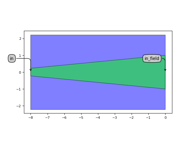
Now with the layout implemented let’s visualize it:
aperture = StripApertureV1()
aperture_lv = aperture.Layout()
aperture_lv.visualize(annotate=True)
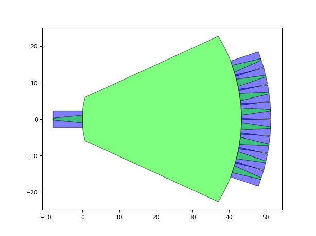
On itself this is a simple component, though an important building block for our star couplers. Let’s verify that our aperture can be used to construct a StarCoupler and check visually that the result corresponds with our expectations.
import numpy as np

N = 12  # number of arms
R = 100.0  # radius of the star couplers
W = 2.0  # aperture width
M = 3  # outputs

# Make a multi-aperture for the arms consisting of N apertures like these, arranged in a circle
angle_step = i3.RAD2DEG * (W + 0.2) / R
angles_arms = np.linspace(-angle_step * (N - 1) / 2.0, angle_step * (N - 1) / 2.0, N)
ap_arms_in, _, trans_arms_in, trans_ports_in = awg.get_star_coupler_apertures(
    apertures_arms=[aperture] * N,
    apertures_ports=[aperture],
    angles_arms=angles_arms,
    angles_ports=[0],
    radius=R,
    mounting='confocal',
    input=True
)

sc_in = awg.StarCoupler(aperture_in=aperture,
                        aperture_out=ap_arms_in)

sc_in_lo = sc_in.Layout(
    contour=awg.get_star_coupler_extended_contour(
        apertures_in=[aperture],
        apertures_out=[aperture] * N,
        trans_in=trans_ports_in,
        trans_out=trans_arms_in,
        radius_in=R,
        radius_out=R,
        extension_angles=(10, 5)
    )
)

sc_in_lo.visualize(annotate=True)
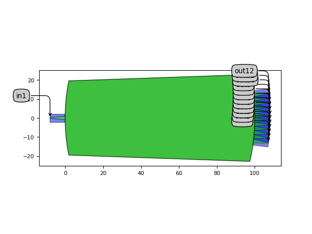
Visually this seems indeed to correspond with what we expect our star coupler to look like. To inspect in more detail we can write the star coupler to a GDS-file and open it in another tool, e.g. KLayout.
sc_in_lo.write_gdsii('star_coupler.gds')
In order for an aperture PCell to be reusable by the StarCoupler component, it needs to meet
a few requirements (just like the one we’ve implemented does).
Important
It must have a trace_template property. This property should have a default value if you don’t want to set it every time you instantiate your aperture.
It must have a aperture_trace_template property. This property should have again a default value if you don’t want to set it every time you instantiate your aperture.
It must have a slab_template property with again a default value.
The aperture port must be placed at (0., 0.) and it must point eastward. That’s why in the example above the start position of our aperture is at x=-transition_length
The ports must be named ‘in’ and ‘in_field’, with ‘in_field’ refering to the port at the aperture side.
RibAperture
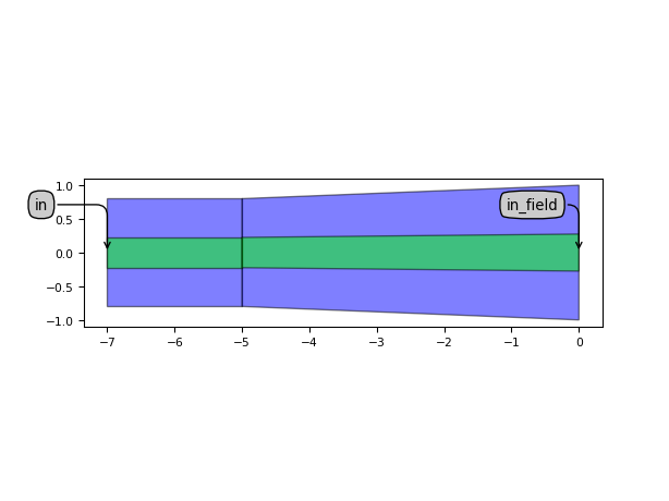
Within these boundary conditions, you’re free to implement as you deem fit. Below we have another example of an aperture, this time we use picazzo’s RibWaveguideTemplate and extend the aperture with a small straight section at the ‘in’ port of the aperture.
from picazzo3.traces.rib_wg import RibWaveguideTemplate, RibWaveguideTransitionLinear

class RibAperture(awg.SingleAperture):
    trace_template = i3.TraceTemplateProperty(locked=True)
    aperture_trace_template = i3.TraceTemplateProperty(locked=True)

    def _default_trace_template(self):
        start_tt = RibWaveguideTemplate()
        return start_tt

    def _default_aperture_trace_template(self):
        end_tt = RibWaveguideTemplate()
        return end_tt

    # if we want to reuse the simulation functionality,
    # we'll need to provide a default for the slab template
    # for now we'll just use as simple template
    def _default_slab_template(self):
        return awg.SlabTemplate()

    class Layout(awg.SingleAperture.Layout):
        """Example of an aperture using a rib waveguide
        """

        # We start with defining parameters
        core_width = i3.PositiveNumberProperty(default=0.45, doc="Core width at start of the aperture")
        cladding_width = i3.PositiveNumberProperty(default=1.6, doc="Cladding width at start of the aperture")
        aperture_core_width = i3.PositiveNumberProperty(default=0.55, doc="Core width at the end of the aperture")
        aperture_cladding_width = i3.PositiveNumberProperty(default=2.0, doc="Cladding width at the end of the aperture")

        def _default_trace_template(self):
            start_tt = self.cell.trace_template.get_default_view(self)
            start_tt.set(core_width=self.core_width, cladding_width=self.cladding_width)
            return start_tt

        def _default_aperture_trace_template(self):
            end_tt = self.cell.aperture_trace_template.get_default_view(self)
            end_tt.set(core_width=self.aperture_core_width, cladding_width=self.aperture_cladding_width)
            return end_tt

        def _generate_instances(self, insts):
            start_tt = self.trace_template
            end_tt = self.aperture_trace_template

            transition = RibWaveguideTransitionLinear(
                start_trace_template=start_tt,
                end_trace_template=end_tt
            )

            straight_length = 2.0
            transition_length = 5.0

            start_straight = i3.Waveguide(trace_template=start_tt)
            start_straight.Layout(shape=[(0, 0), (straight_length, 0.0)])

            lv = transition.Layout(
                start_position=(0.0, 0.0),
                end_position=(transition_length, 0.0),
            )

            insts += i3.SRef(name='start', reference=start_straight, flatten=True)

            insts += i3.SRef(
                name='transition',
                reference=transition,
                # SingleAperture uses self.center to know the center of the aperture
                # this will be used in the simulations
                flatten=True,
            )

            insts = i3.place_and_route(
                insts,
                specs=[
                    i3.Place('transition:out', (0.0, 0.0), angle=0.),
                    i3.Join([
                        ('start:out', 'transition:in'),
                    ])
                ]
            )


            return insts

        def _generate_ports(self, ports):
          # we'll expose the ports of the transition, so that other
          # components can connect to our aperture

          # we map the 'in' port of the transition to 'in'
          # the 'out' port of the transition to 'in_field'
          ports  += i3.expose_ports(
              self.instances,
              {
                  'start:in': 'in',
                  'transition:out': 'in_field',
              }
          )

          return ports

aperture = RibAperture()
aperture_lv = aperture.Layout()
aperture_lv.visualize(annotate=True)
Simulation
Through extending SingleAperture you can integrate into the simulation functionality that comes built in with AWG Designer. AWG Designer provides simulation capabilities for the modes and the free propagation region. These simulations use IPKISS’ virtual fabrication to programmatically generate a 2.5D representation of the component, in which the 3D component is approximated with an equivalent 2D structure of effective indices. The simulation results can be combined into a circuit model that calculates the frequency response of the complete AWG.
Defining SlabModes
If your aperture PCell meets all the requirements listed above, your PCell should be mostly ready to integrate into AWG Designer’s simulation functionality. The only required addition is defining the modes of the slab region. Above we already encountered the slab_template property, but we provided just an empty default. We’ll change that and declare a zeroth order TE-mode, together with a list of neff-values.
from pysics.optics.environment import Environment


# Here we define the mode.
# the neff values can come from experiment or can be obtained with a physical solver.
TE0_mode = awg.InterpolatedSlabMode(
    name="TE0",
    wavelengths=np.linspace(1.2, 1.6, 5),
    n_effs = np.array([3.0568, 2.9866, 2.9223, 2.8617, 2.8042]),
    polarization="TE"
)

# we define the slab template
slab_soi = awg.SlabTemplate(name="SOI_Template")
# the slab layers defined here will be used to construct the camfr simulation of the fields.
slab_soi.Layout(slab_layers=[i3.PPLayer(i3.TECH.PROCESS.WG, i3.TECH.PURPOSE.DF_AREA)])
slab_soi.SlabModes(modes=[TE0_mode])

# use a FieldModel that uses camfr to calculate the fields.
ap = StripApertureV1(slab_template=slab_soi)
ap_sm = ap.FieldModelFromCamfr()

wavelength = 1.55
sim_env = Environment(wavelength=wavelength)
f = ap_sm.get_fields(environment=sim_env, mode=0)
f.visualize()
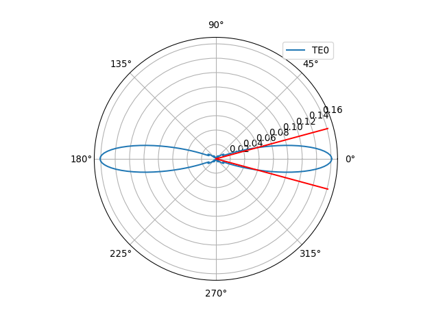
Or we can use the get_far_fields method to calculate and visualize the far field.
ff = ap_sm.get_far_field(environment=sim_env)
ff.visualize()
The FieldModelFromCamfr view we use in the code above, will automatically calculate the fields by performing a simulation on a virtual fabrication of the layout view of the aperture. As a result, when you change the parameters of your aperture, the fields will be recalculated and adapt accordingly.
Defining a custom SlabTemplate
Typically the slabmodes will not change often, hence it’s convenient to create a custom SlabTemplate.
Just like we create trace templates for our waveguides. We can capture the layout and mode information of the slab in a template.
This will make creating slab templates easier.
class CustomSlabTemplate(awg.SlabTemplate):
class Layout(awg.SlabTemplate.Layout):
def _default_slab_layers(self):
return [i3.PPLayer(i3.TECH.PROCESS.WG, i3.TECH.PURPOSE.DF_AREA)]
class SlabModes(awg.SlabTemplate.SlabModes):
def _generate_modes(self, modes):
slab_neff = 2.8
slab_ng = 3.2
# we use 'SimpleSlabMode' here, but could
TE0_mode = awg.SimpleSlabMode(name="TE0", n_eff=slab_neff, n_g=slab_ng, polarization="TE")
return [TE0_mode]
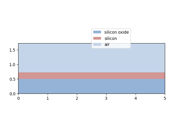
slab_tpl = CustomSlabTemplate()
slab_layout = slab_tpl.Layout()
slab_layout.cross_section().visualize()
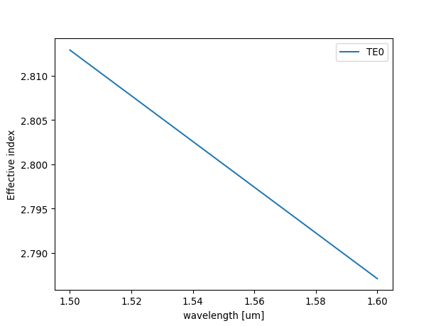
slab_modes = slab_tpl.SlabModes()
slab_modes.visualize(wavelengths=np.linspace(1.5, 1.6, 201))
Before making your own slab template, you should check if the PDK you’re using already contains one. For many of the PDK’s maintained by Luceda, this is the case. If you’re maintaining your own PDK, you can add this class to your own PDK.
With the modes defined, we have now provided all information required for the aperture to feed the right data and simulations into the StarCoupler model.
Customizing Field Calculation
SingleAperture allows you to calculate the fields automatically by first applying the virtual fabrication to the layout view and passing the results to camfr. This approach allows fast iterations, but when you’re looking for more accurate results you might want to rely on experimental data or work with another solver. For this advanced use case it’s possible to extend SingleAperture’s FieldModel view. More specifically we’ll have to implement the get_fields method of view.
For demonstration purposes we’ll implement a simple model that generates a gaussian field for the E0 mode.
Note
We make StripApertureV2 inherit from StripApertureV1, this way we can reuse the layout and we don’t have rewrite it again here. In practice you’ll want to make a single StripAperture PCell.
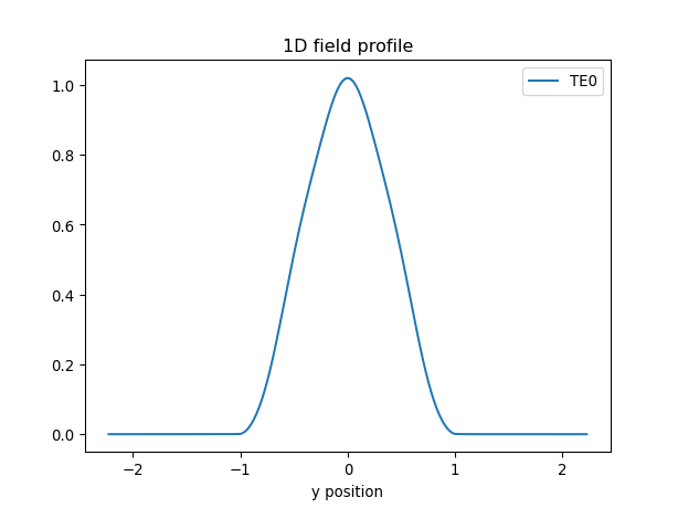
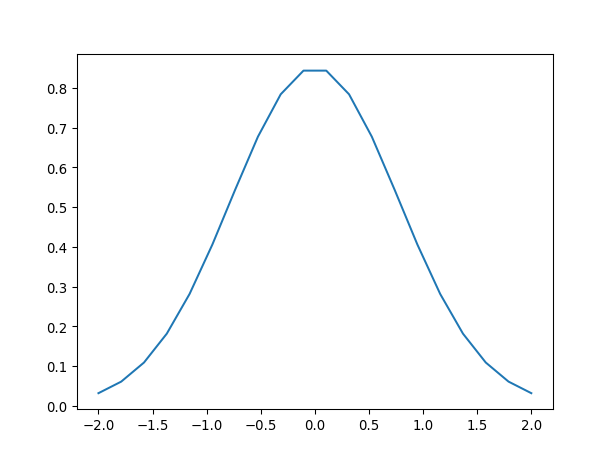
First we use Numpy to write a function that will generate a Gaussian field and visualize it with matplotlib.
import numpy as np

def gaussian_field(waist, x, center=0.0):
    y = np.asarray(x)
    v = np.exp(-((y - center) / waist) ** 2)
    d = y[1:] - y[:-1]
    s = np.cumsum(np.hstack([[0.0], d]))
    norm = np.sqrt(np.trapz(v**2, s))
    return v / norm

mode_waist = 1.1

import matplotlib.pyplot as plt

x = np.linspace(-2, 2, 20)
plt.plot(x, gaussian_field(mode_waist, x))
plt.show()
Now we can use this function to add a FieldModel view to the StripAperture component.
from awg_designer.slabsim import SlabFieldProfile1D
class StripApertureV2(StripApertureV1):
def _default_slab_template(self):
# now that we have our own SlabTemplate, we can set it
# as a default
return CustomSlabTemplate()
class FieldModel(StripApertureV1.FieldModel):
def get_fields(self, mode, environment, verbose=False):
# mode is the index of the mode we use it to retrieve
# the corresponding slab_mode
slab_mode = self.slab_modes[mode]
mode_waist = 1.1
center = self.layout_view.center.y
fields = {
slab_mode.name: gaussian_field(mode_waist, self.positions.y_coords(), center)
}
return SlabFieldProfile1D(
positions=self.positions,
fields=fields
)
StripApertureV2.set_default_view(StripApertureV2.FieldModel)
ap = StripApertureV2()
ap_sm = ap.FieldModel()
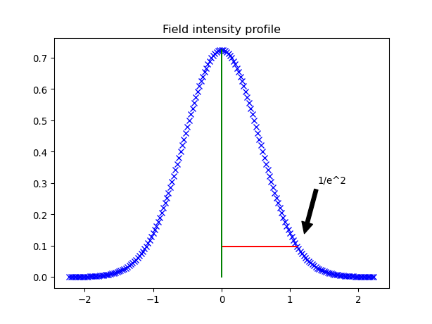
# plot the field intensity profile with the beam waist
wavelength = 1.55
sim_env = Environment(wavelength=wavelength)
f = ap_sm.get_fields(environment=sim_env, mode=0)
near_field_intensity = f.fields['TE0']**2
positions = f.positions.y_coords()
plt.plot(positions, near_field_intensity, 'xb')
plt.plot([0.0, mode_waist], np.ones((2,)) * np.max(near_field_intensity)/np.e**2, 'r-')
plt.plot([0.0, 0.0], [0.0, np.max(near_field_intensity)], 'g-')
plt.annotate('1/e^2', xy=(1.2, 0.13), xytext=(1.4, 0.3),
arrowprops=dict(facecolor='black', shrink=0.05))
plt.title("Field intensity profile")
plt.show()
By implementing the get_fields model, we have now completed our StripAperture component. We have added:
Important
A Layout view, to implement the layout of the aperture
A FieldModel view, to perform the calculation of the fields. Though we could have also used the FieldModelFromCamfr instead.
A custom slab template, to capture the cross sectional information of the slab. This will be used to calculate the fields at the aperture port. Those in their turn feed into the slab simulation.
By inheriting from :py:class`SingleAperture <awg_designer.all.SingleAperture>` we automatically also get a netlist description of our aperture.
With all this set up, our aperture is ready to construct a StarCoupler and construct the corresponding circuit model:
N = 8
ff = ap_sm.get_far_field(environment=sim_env)
div_angle = ff.divergence_angle()
angle = 2 * div_angle # spread angle
angles = np.linspace(-0.5 * angle, 0.5 * angle, N)
ap_width = 3.5
radius = ap_width * N / np.radians(angle)
apm, _, trans_arms, trans_ports = awg.get_star_coupler_apertures(apertures_arms=[ap] * N, apertures_ports=[ap],
angles_arms=angles, angles_ports=[0],
radius=radius, mounting='rowland', input=True)
# Make a star coupler
sc = awg.StarCoupler(aperture_in=ap, aperture_out=apm)
sc_lo = sc.Layout(contour=awg.get_star_coupler_extended_contour(apertures_in=[ap], apertures_out=[ap] * N,
trans_in=trans_ports, trans_out=trans_arms,
radius_in=radius / 2., radius_out=radius,
extension_angles=(10, 10)))
sc_lo.visualize()
# Circuit Model: Calculate the S-matrix of the star coupler
sc_cm = sc.CircuitModel(simulation_wavelengths=None)
wavelengths = np.linspace(1.5, 1.6, 6)
s_matrix = sc_cm.get_smatrix(wavelengths=wavelengths)
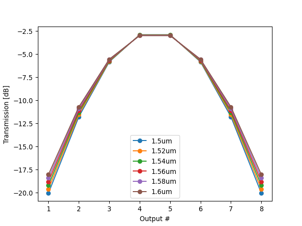
# Plot transmission in the outputs
plt.figure()
for i_wl, wl in enumerate(wavelengths):
t_outputs = [s_matrix["in1", "out{}".format(i)][i_wl] for i in range(1, N + 1)]
plt.plot(range(1, N + 1), 10 * np.log10(np.abs(t_outputs)), 'o-', label="{}um".format(wl))
plt.xlabel('Output #')
plt.ylabel('Transmission [dB]')
plt.legend()
plt.show()

To invoke the slabfield simulation directly and visualize the results, you can execute the code below:
sc_sm = sc.SlabFieldModel()
sim = sc_sm.get_field_simulation(sim_env, 'in1', grid=(0.5, 0.5))
sim.run()
sim.monitors["fields"].get_result().visualize(overlays=[sim.space])
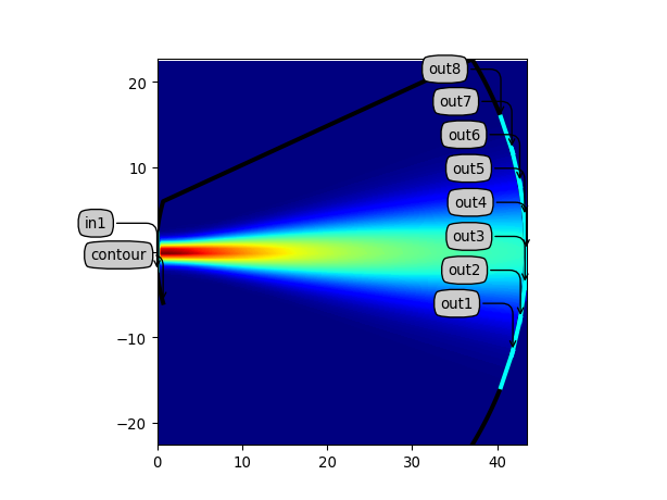
Our aperture contains both a camfr field model as well as our custom model that uses the gaussian_field function. This allows to compare the 2 methods and inspect the differences between them.
ap = StripApertureV2()
ap_sm = ap.FieldModelFromCamfr()

apm, _, trans_arms, trans_ports = awg.get_star_coupler_apertures(apertures_arms=[ap] * N, apertures_ports=[ap],
                                                          angles_arms=angles, angles_ports=[0],
                                                          radius=radius, mounting='rowland', input=True)

# Make a star coupler
sc = awg.StarCoupler(aperture_in=ap, aperture_out=apm)

sc_lo = sc.Layout(contour=awg.get_star_coupler_extended_contour(apertures_in=[ap], apertures_out=[ap] * N,
                                                             trans_in=trans_ports, trans_out=trans_arms,
                                                             radius_in=radius / 2., radius_out=radius,
                                                             extension_angles=(10, 10)))

sc_cm = sc.CircuitModel(simulation_wavelengths=None)
wavelengths = np.linspace(1.5, 1.6, 6)
s_matrix = sc_cm.get_smatrix(wavelengths=wavelengths)

# Plot transmission in the outputs
plt.figure()

for i_wl, wl in enumerate(wavelengths):
    t_outputs = [s_matrix["in1", "out{}".format(i)][i_wl] for i in range(1, N + 1)]
    plt.plot(range(1, N + 1), 10 * np.log10(np.abs(t_outputs)), 'o-', label="{}um".format(wl))

plt.xlabel('Output #')
plt.ylabel('Transmission [dB]')
plt.legend()
plt.show()
sc_sm = sc.SlabFieldModel()
sim = sc_sm.get_field_simulation(sim_env, 'in1', grid=(0.5, 0.5))
sim.run()
sim.monitors["fields"].get_result().visualize(overlays=[sim.space])
