Introduction to Python
Note
The following people contributed to this tutorial: Yannick De Koninck, Emmanuel Lambert, and Gunay Yurtsever (Ghent University)
Python is a high-level programming language suited for applications from simple automation tasks to full-blown software frameworks. This guide will teach you some of the basics of the Python language and its standard libraries, which you need to know to be able to use the Luceda software.
Python essentials
In this section you will learn about:
Variables
Lists and arrays
Loops
Functions
Loading modules
To illustrate this, we will construct a script to estimate the value of pi by means of a series approximation.
First, create a new script calculate_pi.py and open it.
The first thing we should do is greet our users. We can do this using the print command. Add the following code to calculate_pi.py:
print("Welcome to the Python pi-calculator")
print("-----------------------------------")
This will print the greeting to screen and underline it. Be aware that each print statement automatically starts at a new line. We’re now ready
to start learning about variables.
Variables
Defining variables in Python is remarkably easy. Unlike in other languages, such as C, you don’t need to tell the type of the variable to Python, you just assign a value to it. So, say you want to define a variable called a that holds the number 7, you just write:
a = 7
Python will figure out for you that a is a number. If you’re familiar with Matlab or Javascript, then you’re already familiar with this programming style.
Let’s put this into practice. We’ll calculate pi using a series approximation, so we’ll need a variable to hold the number of terms we will retain. We also need an initial value for our pi-estimate, which is zero.
Underneath the two print statements, add the following code:
pi_estimate = 0.0
terms_in_series = 5000000
Notice that we explicitly tell Python that pi_estimate is a floating point number, by adding .0 to its value, and that terms_in_series is an
integer number. It is good practice to always do this because arithmetic operations on both types differ in Python (version 2): e.g. 2/5 yields 0 and 2.0/5.0 yields 0.4.
Lists and arrays
Numbers are nice, but often you will need a variable to hold a series of numbers, for example measurement data or results of a simulation sweep. You can save these values in so-called lists. They are initiated using square brackets and elements are separated by commas (,). An example (you don’t have to add this to the sample code):
a = [1, 2, 3]
b = [4, 5, 6]
You can access individual elements using the square bracket syntax you are used to from for example C:
print(a[1])
will print 2 to the screen. Remember that the first element has index 0!
Lists are great to store data but difficult to perform arithmetic operations on. If you write:
c = a + b
then c will be:
[1, 2, 3, 4, 5, 6]
instead of the piecewise sum of elements.
If you want to be able to perform arithmetic operations, you should use numpy arrays. We are running a little ahead here since we did not introduce numpy yet, but that doesn’t matter at this point. All you have to know is that if you write:
a = array([1, 2, 3])
b = array([4, 5, 6])
c = a + b
then c will be:
[5, 7, 9]
It is useful to know that numpy (again, we’ll talk about numpy in a minute) has a few helper functions to instantiate arrays, such as:
zeros(N): create an array of length N filled with zeros
ones(N): create an array of length N filled with ones
Loops
In scientific computing you will encounter a lot of situations where you have to repeat the same operation on a large number of objects, like manipulating a set of measured values or repeating simulation for an entire wavelength range. In either case, you will want to use a loop to iterate over the involved objects. In python this is done by iterating over a predefined list and looks like this:
for element in some_list:
    do_something(element)
Where some_list is a list of values and element is the next value in that list for iteration. In other words, if some_list were
e.g. [0, 12, 4], the value of element would be 0 during the first iteration, 12 during the second and 4 during the last. In that case, the
for-loop would be equivalent to:
do_something(0)
do_something(12)
do_something(4)
Two important aspects of the structure of the for loop are the presence of the colon (:) and the indentation. The colon indicates the
beginning of the body of the for loop, and each statement inside this body should be indented by one tab from the for .. in ..: statement itself.
Another example:
for element in some_list:
    do_something(element)
    do_something_else(element)
    do_even_more_stuff(element)

do_something_outside_the_loop()
In this case, the first three statements are executed during each iteration of the loop, and the last statement is executed after the loop has finished iterating. So remember: indentation is very important in Python!
Let’s use this knowledge to calculate the series expansion of pi. The series expansion of pi reads:
To implement this, add the following line under the variable definitions:
for k in range(terms_in_series):
    pi_estimate = pi_estimate + 4.0 * (-1)**k / (2*k+1.0)
We don’t have a predefined list so we create it inside the for-statement. The function range(some_integer_number) generates a list of
integers starting from zero and ranging to some_integer_number-1, so the list will hold some_integer_number elements. As discussed before, the
value of k will iterate through this list hence its value will be 0 during the first iteration, 1 during the second, and so on, all the way to terms_in_series-1.
During each iteration, our estimate is further refined by adding one more term to it.
What’s left now is to print the approximate value of pi to the screen. Add this print statement underneath the for-loop, but make sure the indentation is correct, as we discussed before.
print("Pi is approximately {0}".format(pi_estimate))
The construct "some string with substitution placeholders {0} and {1}".format(some_value, or_some_other_object) allows to generate a string with
a representation of numbers or other python objects inside the string, using substitution placeholders. The {0} will be substituted by the first
parameter of format, in this case pi_estimate, and so forth.
The entire program should look exactly like this at this point:
print("Welcome to the Python pi-calculator")
print("-----------------------------------")

pi_estimate = 0.0
terms_in_series = 5000000

for k in range(terms_in_series):
    pi_estimate = pi_estimate + 4.0 * (-1)**k / (2*k+1.0)

print("Pi is approximately {0}".format(pi_estimate))
You can run the program now, and it should output:
Welcome to the Python pi-calculator
-----------------------------------
Pi is approximately 3.14159245359
Functions
A function is a piece of logic that takes a number of variables (the ‘arguments’), does something to them or based on them, and usually returns a result. By putting an algorithm which is re-used several times in your program inside a function, you can write it only once and then re-use. You can define a function like this:
def my_function(argument1, argument2):
    do_something(argument1)
    do_something_else(argument2)
    return the_result
The def keyword indicates the start of the function definition, followed by its name and a list of arguments, separeted by commas and enclosed between brackets.
Notice the use of the colon (:) and the indentation scheme we already learned about in the previous section about the for-loop.
Time to put this in practice. It might seem like overkill, but just to illustrate the use of functions, let’s implement the actual calculation of pi in a separate function. Change your code to this:
def calculate_pi(terms_in_series=10000):
    pi_estimate = 0.0
    for k in range(terms_in_series):
        pi_estimate = pi_estimate + 4.0 * (-1)**k / (2 * k + 1.0)
    return pi_estimate

print("Welcome to the Python pi-calculator")
print("-----------------------------------")

terms = 5000000
pi_est = calculate_pi(terms_in_series=terms)

print("Pi is approximately {0}".format(pi_est))
The function to calculate pi is defined at the top of the script. It takes 1 argument, terms_in_series, and we give it a default value of 10000.
You don’t have to do that, you could also just write:
def calculate_pi(terms_in_series):
but specifying a default value allows you to call the function without providing that argument, in which case pi will be calculated retaining the first 10000 terms in the series.
pi_est = calculate_pi()
If you’re not happy with the default value, you specify the value you want like this:
terms = 5000000
pi_est = calculate_pi(terms)
The best way, though, is to explicitly mention the name of the argument you want to set, like we did in the example:
terms = 5000000
pi_est = calculate_pi(terms_in_series=terms)
Loading modules
In many cases you need to do much more advanced stuff than adding two numbers and printing the result to the screen. In section 3 of this tutorial we will implement a python program that calculates Fourier transforms of signals and draws these to the screen. These advanced functions, such as calculating ffts and plotting graphs, are readily available in Python through so-called modules. For generic scientific computing, three libraries with such modules will prove to be very convenient:
numpy: basic numerical computing such as matrix manipulations, linear algebra and Fourier transforms
scipy: more advanced numerical functionality such as statistics, signal processing and image processing
matplotlib: powerful plotting library which allows to plot both 2D and 3D datasets
A module is loaded using the import statement, which you can use in a few different manners:
from module_name import *
from module_name import function1, function2
import module_name
import module_name as mn
The first statement loads all the functions that are available in the module module_name, so you can start using all the functions without any
further ado. This approach is not generally advised however, since it pollutes your local namespace - all the functions which you don’t need will
also be available in your program, which can slow down the execution. The second form illustrates how to import only selected functions.
The third line also gives access to all the functions in the module, but does not pollute the local namespace. You then need to mention the module name each time you use a function in it. So, if you want to call function1 inside module_name, you have to write:
module_name.function1()
Finally, the last form does the same as the third but specifies a shorthand for the module name, so it becomes less tedious to use:
mn.function1()
This last approach is preferred, in particular for standard libraries including ipkiss:
import ipkiss3.all as i3

L = i3.Library(name="my_design_library")
Let’s add two more features to our pi calculation program using functionality in external libraries. First of all we could measure the time we need
to calculate pi and second we can compare our result to the more exact value and calculate the relative error. The constant pi is hard-coded in
the numpy library and time can be measured using a library called time. Add the following lines to the top of our script, above the function definition:
import time
import numpy as np
and add the following line before the call to the calculate_pi function:
start_time = time.time()
The time() function returns how many seconds have elapsed since January 1, 1970 - if you want to know why then search for ‘unix’ and ‘epoch’ using
your favorite search engine. This will provide our reference moment in time.
Next, add these two lines immediately after the calculate_pi call:
duration = time.time() - start_time
relative_error = abs(pi_est - np.pi) / np.pi
We calculate the elapsed time by subtracting the reference time from the current time. The relative error is calculated by comparing our estimate to the hard-coded value of pi in numpy.
Finally, print the newly calculated information to the screen by adding the following statements at the end of the file:
print("Relative error: {0}".format(relative_error))
print("Calculation done in {0:.3f} seconds".format(duration))
The last statement adds a format specifier to the substitution specification, saying that the number should be printed as a fixed point number with 3 digits after the point.
The entire program should now look like this:
import time
import numpy as np

def calculate_pi(terms_in_series=10000):
    pi_estimate = 0.0
    for k in range(terms_in_series):
        pi_estimate = pi_estimate + 4.0 * (-1)**k / (2 * k + 1.0)
    return pi_estimate

print("Welcome to the Python pi-calculator")
print("-----------------------------------")

terms = 5000000

start_time = time.time()
pi_est = calculate_pi(terms_in_series=terms)

duration = time.time() - start_time
relative_error = abs(pi_est - np.pi) / np.pi

print("Pi is approximately {0}".format(pi_est))
print("Relative error: {0}".format(relative_error))
print("Calculation done in {0:.3f} seconds".format(duration))
and output something like:
Welcome to the Python pi-calculator
-----------------------------------
Pi is approximately 3.14159245359
Relative error: 6.36619815147e-08
Calculation done in 1.953 seconds
Object Oriented Programming in Python
What is object oriented programming
In this section you will learn:
What object oriented programming is
How to define classes in Python
How to use your newly created class
What inheritance is and how to use it.
The program we wrote in the previous section was short and simple. In everyday science and engineering you will encounter larger problems that require more sophisticated computer programs. Soon, it will become very difficult and cumbersome to solve your problem using one piece of code in one file like we did. You will want to split up your problem in logical entities, each dealing with a smaller part of the problem. For example, in this section we will elaborate a program that adds noise to a clean signal and filters the disturbed signal in order to recover the original signal again. At first glance it might seem doable to implement this problem in the same way we did before. But what if, sometime in the future, you decide you want to extend the program to simulate a communication channel? You want to modulate the signal with a bitstring, simulate the transmission of that signal over a fiber optic channel, filter it again and try to recover the bitstring at the receiver’s end. In this case splitting up your program in smaller pieces from the beginning will save you a lot of time and mistakes. If you do do not really get the difference now, read this paragraph again after you’ve finished this section.
Secondly, a wide range of programming problems, including IC design, lend them selves to a programming “paradigm” in which there are objects which you can act upon. One can define types of objects, with the functions that can act on them. This is what we call object oriented programming (well, at least the gist of it…)
Splitting up your problem using object oriented programming is done by means of classes. If you have experience with programming languages like C++ or Java you will certainly have heard about classes before. A class is an entity (something) which specifies the ‘type’ of an object (another ‘something’) that has two things: some data and methods. In other words: a class specifies a certain type of object which has things and can do things. We could for example define a class called Person. This class will specify the data, like the person’s birthday, his/her name, the color of his/her hair, his/her length, a list of his/her friends and so on. This person class will also have a number of methods, like: walk, eat, sleep, go to the grocery store, … So remember, every object has a type, a class, which specifies the data an object and the methods that a certain object has.
Everything in python is an object with a certain class. Even classes have a type, a metaclass, but that would lead us way too far.
Object Oriented Programming in Python
To make this a little more concrete, let’s take a look at another example of what a class could look like. Consider a sampled signal over time. Such a signal has some properties, like the list of its values at the different sample-times, the length of the signal in seconds, the sample rate. There are also some things you can do to a signal, like calculating its Fourier spectrum or plotting it to the screen. Let us translate this into python code.
First, add a new file to the project which will hold the code for our signal class and name the file signals.py. Add the following lines to it:
import numpy as np

class Signal(object):
    def __init__(self, value_array, sample_rate=1000):
        self.sample_rate = sample_rate
        n_o_samples = len(value_array)
        length = float(n_o_samples) / float(sample_rate)
        self.time_steps = np.linspace(0, length, n_o_samples)
        self.values = np.asarray(value_array)

    def get_sample_rate(self):
        return self.sample_rate
Let’s take a closer look at this code snippet. The first line (after the import statement) tells Python that we are going to define a class which
we want to call Signal and which inherits from object. Don’t bother about inheritance yet, we’ll talk about it in the next section. Just remember that this
first line initiates the class definition. Notice again the colon (:) sign and the indentation scheme used to specify what code is part of the class
definition and what part is not.
The second line of code defines a function called __init__. This is the so-called constructor and will be called when an object of this class
is created. Three arguments are passed: self, value_array and sample_rate. The self argument (always the first one) is the object that
will hold all the data of that class. You can look at it as if it were a box where you can put all the information regarding the object. We’ll see
in a minute how that works. The second argument is an array of sampled values of the signal we wish to define. The third and final argument is
the sample rate at which the signal was sampled. It is set to 1kHz by default, but users of our class can set their own sample rate if it deviates
from the default values.
Inside the constructor method some attributes of the class are set on the self argument. This ensure we will be able to access these variables
in other methods of the class, as we will see later. In our code snippet the sample rate is copied from the value passed as an argument, and an array of
time-steps is created using the linspace function from numpy. This function generates an array of length no_o_samples ranging from 0 to length.
These are the timesteps at which the samples of our signal were taken. Finally the values of the signal at each timestep are saved to self.values
by converting them to a numpy array using the asarray function.
We also define a second method, called get_sample_rate. This method doesn’t take any arguments but returns the sample rate of the signal, which will
be useful later.
So now you will be able to create an object of the type Signal like this:
sig = Signal(value_array=vals, sample_rate=20000)
Assuming vals is an array of values, this line of code will initialize sig as a Signal that has samples values vals at a sampling rate
of 20kHz. We won’t be using this in our code yet but this just shows you how to do it.
But our Signal class as it is now is pretty useless so let’s add a method that calculates the Fourier transform of a signal. The code for calculating
the fft of an array of values resides in the numpy.fft module, so below numpy’s import statement, add:
import numpy.fft as fft
Next, add the following lines below the get_sample_rate() method, at the same indentation level:
def get_fft(self, shifted = True):
    ft = fft.fft(self.values)
    freqs = fft.fftfreq(len(self.values), self.time_steps[1])

    if (shifted):
        ft = fft.fftshift(ft)
        freqs = fft.fftshift(freqs)

    return [freqs, ft]
The get_fft function takes 2 arguments, the self parameter that holds the object, and an optional shifted parameter. The method for
calculating the fft of an array of values returns the fft signal in a special format: first the values for frequencies from 0 to F/2,
followed by the values from -F/2 to the one before 0. In most cases you want the order of the fft-values to be arranged from -F/2 to F/2, t
his can be done using fftshift, called when shifted is true. This method also calculates the frequencies corresponding to the Fourier
components. Notice how the object’s attributes self.values and self.time_steps are called. The function returns 2 one-dimensional arrays,
the first containing the frequencies at which the fft values are calculated and second the fft-values themselves.
So now let’s take a look at how you could use this (you don’t have to add this to your code, this is just for illustration). Again, vals
is an array of values, e.g. from a measurement:
sig = Signal(value_array=vals, sample_rate=20000)
f,ft = sig.get_fft()
It’s that simple!
Before we go any further adding functionality to our class, we should talk about inheritance first. It’s one of the coolest features object oriented programming has to offer!
Inheritance
Let’s go back to the end of paragraph What is object oriented programming, where we talked about how “Person” could be a class. It has properties (data) and it can do stuff. Now we want to make a class “Person_that_works_in_a_company” or maybe better “Employee”. An Employee has properties (e.g. salary) and does stuff (e.g. go to work, do some work) that other people don’t do, but the class should also support all the functionality we already programmed for the Person class. What we could do is copy the code we wrote for the Person class into the Employee class and add some extra. But this will turn out to be a very bad idea! What if you want to edit some parts of the Person class? In that case you would have to correct both classes, making sure you don’t make any mistakes. Soon you’ll discover that you did make mistakes and have a hard time to keep your code running properly. Luckily Python supports inheritance. This is a technique that allows to reuse the code you wrote before and simply add or modify the parts that you need. This is very vague, so let’s take a look at how this could work.
The signal class that we started building is for general signals, but say we will be working with sine signals a lot and want to write a class for them. Instead of providing an array of values, we want to initialize this by passing through the sine frequency and the amplitude, so our constructor function will be completely different. On the other side we want to be able to calculate the Fourier transforms using the code we already wrote. So the sine class should inherit all the functionality from the signal class. At the bottom of signal.py, at the same indentation level as the Signal class definition, add the following code:
class SineSignal(Signal):
    def __init__(self, signal_frequency=0.25, length=0.5, sample_rate=1000.0):
        self.time_steps = np.linspace(0, length, int(length*sample_rate))
        self.sample_rate = sample_rate
        self.values = np.array( [ np.sin(2 * np.pi * signal_frequency * t) for t in self.time_steps])
We defined a new class called SineSignal. After the name of the new class we see Signal between brackets. This means that
SineSignal inherits from Signal. We define a new __init__ method that overrides Signal’s constructor. Instead of passing through
an array of values, the user optionally provides the sine frequency and amplitude along with the sample rate. The list of values is generated
inside the constructor using the following piece of code:
[ np.sin(2 * np.pi * signal_frequency * t) for t in self.time_steps]
This construction is called a generator. A list of values is generated base on the sin function from numpy, where each value in the new list is created using a value in the self.time_steps array. Next this list is casted to an array and assigned to self.values.
Now we can generate a sine signal like this:
sine = SineSignal(signal_frequency=70.0)
but still use the methods we wrote for the Signal class off the shelf:
f, ft = sine.get_fft()
This is the power of inheritance.
Intermezzo: plotting in Python
There are no plotting tools built right into Python, but for scientific plotting we use a package called matplotlib. The usage of this module is very similar to plotting in MATLAB. To draw e.g. a 2D plot you write:
plot(x_axis_values1, y_axis_values1)
plot(x_axis_values2, y_axis_values2)
xlabel("This text will appear under the x-axis")
ylabel("This text will appear next to the y-axis")
show()
The parameters in the plot() statements are arrays containing the x- and y- values. In this case 2 different graphs will be drawn on
the same axes, because there are 2 plot statements. You can add axis labels using the xlabel() and ylabel() functions. The show() statement
will actually draw the plot to the screen.
Matplotlib has a very clear reference guide at matplotlib.org, where you will
find a list of all the available functions and how to use them.
Let’s implement this feature into our Signal class. First, load the Matplotlib module by adding this line below the other two import statements:
import pylab as plt
Underneath the get_fft() method definition, at the same indentation level, add the following code:
def plot_values(self):
    plt.xlabel('time (s)')
    plt.ylabel('signal value (a.u.)')
    plt.plot(self.time_steps, self.values)
Nothing new here. We don’t include the show() statement yet because the user might want to combine different plots on the same graph.
Using your classes
So we have built a signal class, we implemented methods to calculate the Fourier transform and plot the signal, and defined a sine signal class that inherits from the basic signal class. Time to stitch everything together in a main script. Create a new script file called main_signal.py.
Add the following lines to it:
import signals as sig
import pylab as plt

print('Welcome to our signal filtering program')
print('---------------------------------------')

print('Generating signals...')
sine = sig.SineSignal(length=2.0)

print('Plotting...')
sine.plot_values()
plt.show()
First, our signals module and matplotlib are loaded. Our module is called signals because the file that contains the class definitions is called signals.py. (Make sure you
didn’t call your file signal.py, or you will induce a conflict with a standard python module).
Run the script. If everything went well, you should see something like:
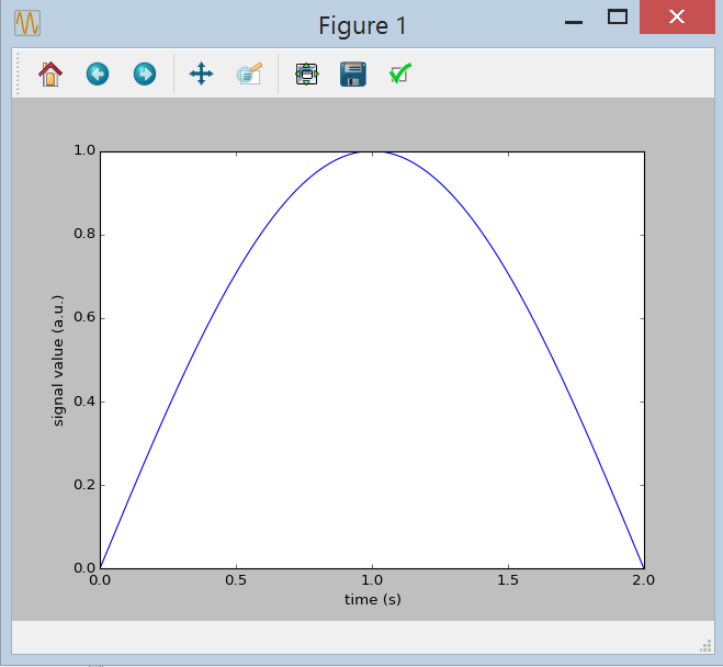
Plot of our sine signal
You can use the different controls on top of the window (or below, depending on your version of matplotlib) to pan around and zoom in and out. Close the window after you finished inspecting the signal plot.
Advanced class features
We’ve learned about object oriented programming and wrote a basic signal class. In this section we’ll add some more advanced features to the class and learn about:
Private methods
Method overloading
Operator overloading
Private methods
When writing a class you might encounter situations where you want to write a helper method that you use a lot inside your class definition but that shouldn’t be accessible for people that use the class. In this case you will want to use private methods, which are only accessible inside the class definition. You can indicate a method as private by adding an underscore character before the name of the method:
class SomeClass(object):
    def _this_is_a_private_method(self):
        do_something()
        return
No time to waste, let’s use it in our Signal-class. We’ll implement a more advanced plotting method that plots
the signal and its Fourier image in 1 window on two different graphs. For that we’ll define two private helper method,
one that plots the signal itself and another one that plots the Fourier image.
Make the plot_values() method private by adding an underscore character before its name and add the following code below:
def _plot_fft(self):
    [ freqs, ft ] = self.get_fft()
    plt.xlabel('Frequency (Hz)')
    plt.ylabel('Fourier Component (a.u.)')
    plt.plot(freqs,ft)

def plot_signal(self, plot_title = 'Unnamed signal'):
    fig = plt.figure()
    fig.subplots_adjust(hspace = 0.38)
    plt.subplot(2,1,1)
    plt.title(plot_title)
    self._plot_values()
    plt.subplot(2,1,2)
    plt.title('Spectrum')
    self._plot_fft()
The _plot_fft() method is nearly identical to _plot_values(). The plot_signal() method starts
by creating a new figure i.e. a new window. The second line is a mere technicality, telling
matplotlib to increase the vertical space between two plots in a single window to 0.38 units. The third statement,
plt.subplot(2,1,1) indicates that we want the window to be divided into 2 (first argument) rows and 1 (second argument)
column and that the next plot should be on the first (third argument) axes (which is the upper one).
This is very similar to how you use subplots in MATLAB. Next, a title is set for that plot (passed as an optional argument)
and the signal itself is drawn using the private method. This is repeated for plotting the fft image.
Now run the main file again.
Whoops! An error occurred:
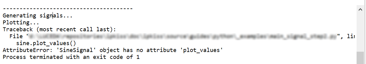
Remember we renamed the method to make it private. (However, single underscore is just a convention in python. If you want to make the method actually inaccessible, add double underscores: __really_private_method()). We defined a new method, plot_signal(), so let’s replace sine.plot_values() in the main file to:
sine.plot_signal(plot_title='Sine signal')
Running the main file now should yield=
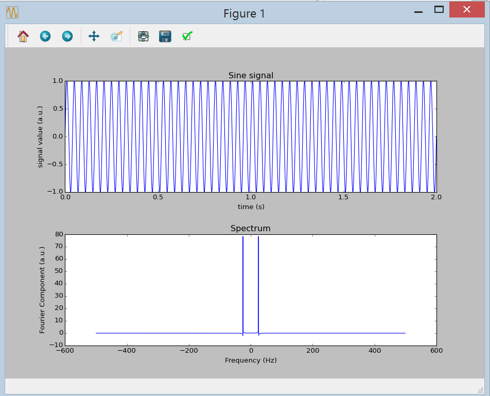
Operator overloading
Overloading operators is something you won’t be using a lot, but in this project it is very convenient and implementing it is a piece of cake. We want to be able to use the + (plus) operator between two objects of the signal class to generate a new signal who’s value array is the sum of the value arrays of the two signals that were summed, the behavior you would expect from adding two signal objects together.
Within Python, you can define how operators like +, -, * and so forth should behave on a certain type. This is used within IPKISS to implement syntax like:
s1 = i3.Shape([(0.0,0.0), (10.0,0.0)])
s2 = i3.Shape([(20.0,10.0), (30.0,30.0)])

s_full = s1 + s2
So after reading this section you know how this works!
To overload the plus (+) operator, you have to add the method __add__(self, signal), which returns self + signal. The implementation of
this method is straightforward: add the following code after the constructor (__init__()) in the Signal class definition:
def __add__(self, signal):
    if (len(signal.values) != len(self.values)):
        raise Exception("Error in Signal: __add__: length of 'signal.values' ({}) parameter differs from length of 'self.values' ({})".format(len(signal.values), len(self.values)))

    ret_sig = self.values + signal.values
    return Signal(ret_sig, self.sample_rate)
First we check if both signals have the same length, if they don’t then we throw an exception. This means that the program will stop running
and an error message will appear in the terminal. If the value-arrays have equal length, a new value array ret_sig is created that is the sum of the two value arrays.
It is always good practice to include as much information in your error description as you can. The error message itself is formatted using the
string formatting syntax that we used before. Finally a new signal object is instantiated using the new value array and the sample rate.
It wouldn’t be a bad idea to check if the sample rates are equal and raise an exception if they aren’t - this is something you can try to implement yourself.
You can test your overloaded operator by substituting sine = sig.SineSignal(length=2.0) in the main file with:
sine = sig.SineSignal(length = 2.0) + sig.SineSignal(signal_frequency = 70.0, length = 2.0)
Plotting this will yield:
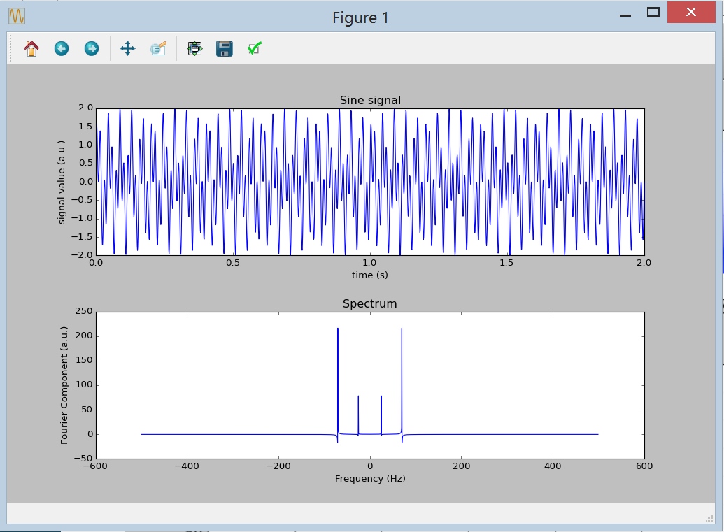
Addition of two sine signals using overloaded + operator
You can easily distinguish the two different sinusoidal components in the Fourier image.
You can restore the sine assignment to its previous state:
sine = sig.SineSignal(length=2.0)
This finishes up our Signal class definition.
Finishing the sample program
All that is left now is to define another subclass that can generate white noise and write a small class that implements the filter. We will not introduce many new concepts from now on but rather show you how the object oriented approach can help you to write clean programs.
Adding the Noisy Signal class
Adding the Noisy Signal subclass is similar to the Sine signal subclass, but instead of the sine function we use a random number generator that is available through the numpy.random module. Import this module by adding this line at the top of Signal.py
import numpy.random as rnd
Add the following code below the Sine class definition:
class NoisySignal(Signal):
    def __init__(self, length=0.5, sample_rate=1000, amplitude=1):
        self.time_steps = np.linspace(0, length, int(length*sample_rate))
        self.sample_rate = sample_rate
        self.values = 2.0 * amplitude * (rnd.random(size=(len(self.time_steps),))-0.5)
As you can see, the np.sin() function call is replaced by rnd.random() which generates an array of uniformly distributed random numbers. The random() function
takes an argument which is the size of the array to be generated (in this case we tell it to generate a one-dimensional array of size self.time_steps). It returns
random values in the interval [0,1[. We rescale it to have the correct amplitude and center it around 0.0 by subtracting 0.5.
Let’s add a noisy signal to our sine signal and plot both. In main.py, add the following line after the sine signal is generated:
noise = sig.NoisySignal(length=2.0)
dirty_signal = sine + noise
and add the following line after the plotting command for the sine signal:
dirty_signal.plot_signal(plot_title = 'Dirty Signal')
Running the program will show 2 windows (remember we called figure() before each signal plot), the first one drawing the
clean signal, the second one the dirty signal:
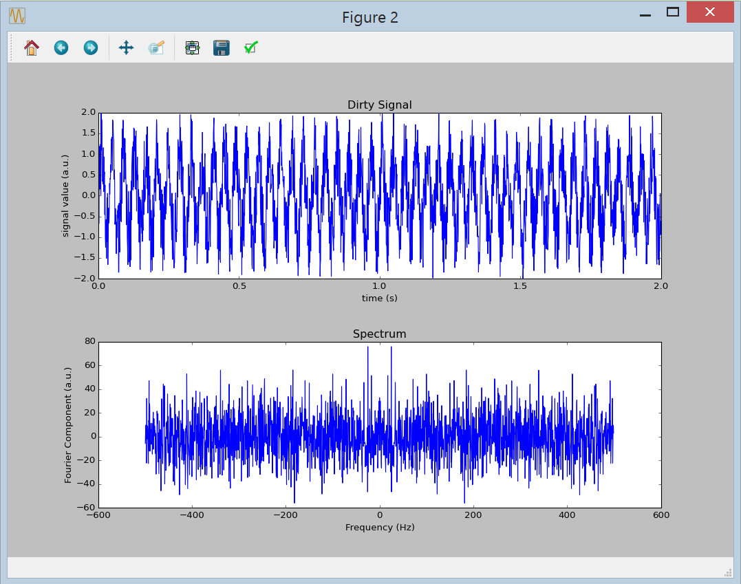
Sine with noise added
Implementing the filter class
Next we’ll add a class that filters a signal by multiplying the Fourier image of that signal with a window of a certain width and center frequency. First add a new file to the project called signal_filter.py.
First add the following import statements at the top of the new file:
import signals as sig
import numpy.fftpack as fft
import numpy as np
We’ll be using our signals module, the fftpack and numpy.
Next, add the following lines below the import statements to start the Filter class definition:
class Filter(object):
    def __init__(self, center_frequency, bandwidth):
        self.lower_bound = center_frequency - bandwidth/2.0
        self.upper_bound = center_frequency + bandwidth/2.0
The user passes through the center frequency and bandwidth of the window filter, but for calculating the frequency response, we are only interested in the lower and upper frequency bounds of the pass band, so we save these to self. You will now understand what the object between brackets after the class name means: the class inherits from the generic object class, which all new classes in Python inherit from.
The filter class has one more method we need to implement: the filter_signal method that takes a signal and returns a filtered signal. Add the following code below the constructor:
def filter_signal(self, signal):

    [freqs, fourier_signal] = signal.get_fft(shifted=False)

    n_o_samples = len(freqs)
    freq_filter = np.zeros(n_o_samples)
    filtered_fourier_signal = np.zeros(n_o_samples, dtype=complex)

    for i in range(n_o_samples):
        if (np.abs(freqs[i]) > self.lower_bound) and (np.abs(freqs[i]) < self.upper_bound):
            filtered_fourier_signal[i] = fourier_signal[i]
        else:
            filtered_fourier_signal[i] = 0.0 + 0.0j

    filtered_signal = fft.ifft(filtered_fourier_signal)

    return sig.Signal(value_array = filtered_signal, sample_rate = signal.get_sample_rate())
By now you should be able to understand the code here. A few comments though:
The
np.zeros()call contains an argument calleddtype, which defines the datatype of the elements in the array, in this case complex numbers since the Fourier transform of a real signal is in general complexAs you can see, you can hard-code complex numbers by using
jfor the imaginary part
Adjusting the main file
Finally, let’s use the new filter class to clean up the dirty signal. In the main file, first import the Filter class by adding the following import statement below the existing import statements in main.py:
import signal_filter as fil
Below the line of code where we sum the sine and noise signal, add the following lines:
print('Generating filter..')
pass_filter = fil.Filter(center_frequency=25.0, bandwidth=2.0)

print('Filtering..')
cleaned_signal = pass_filter.filter_signal(dirty_signal)
We create a band-pass filter of center-frequency 25.0 Hz and bandwidth of 2.0 Hz. Next we apply the filter to obtain a cleaned up signal. All that is left is to plot the cleaned up signal. Add the following line after the code to plot the dirty signal:
cleaned_signal.plot_signal(plot_title='Cleaned signal')
Now run the code. You will find the previous two plots along with a new plot showing the cleaned-up signal:
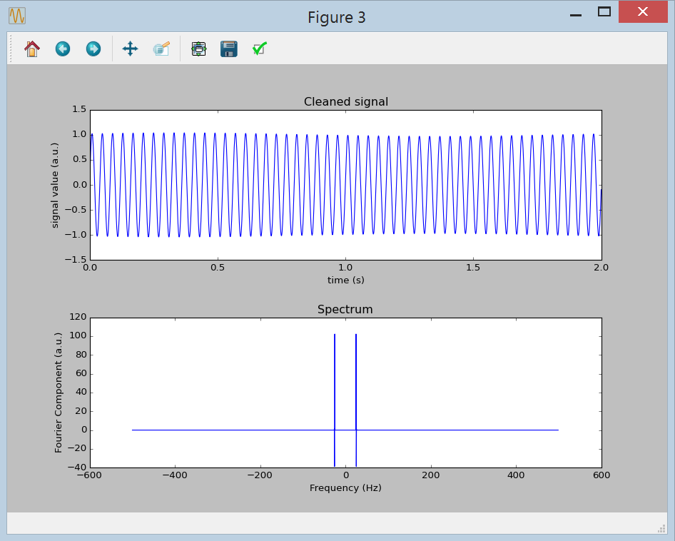
Filtered sine with noise signal
This concludes our basic tutorial on Python. By now you should be able to understand and write basic Python code. Congratulations!