WG1

class ipkiss3.cml.WG1(**kwargs)

Single mode waveguide model with a linear dispersion curve.

Parameters

n_eff: float

Effective index at center_wavelength.

n_g: float

Group index at center_wavelength.

loss: float (dB/m)

Loss of the waveguide in dB/m.

center_wavelength: float (m)

Center wavelength (in meter) of the model at which n_eff, n_g and loss are defined.

length: float (m)

Total length of the waveguide in meter.

Notes

The actual effective index is a linear function of wavelength, and calculated as follows:

\[n_{eff}(\lambda) = n_{eff,0} - (\lambda-\lambda_c) * \frac{n_g-n_{eff}}{\lambda_c}\]

Where \(\lambda_c\) is the central wavelength, at which \(n_{eff}(\lambda_c)=n_{eff,0}\).

The scatter matrix is given by:

\[\begin{split}\mathbf{S}_{wg}=\begin{bmatrix} 0 & \exp(-j\frac{2 \pi}{\lambda}L n_{eff}(\lambda)) * A \\ \exp(-j\frac{2 \pi}{\lambda}L n_{eff}(\lambda)) * A & 0 \end{bmatrix}\end{split}\]

Where the amplitude loss is calculated as:

\[A = 10^{-loss_{dB/m} * L/20.0}\]

Terms

Term Name	Type	#modes
in	Optical	1
out	Optical	1

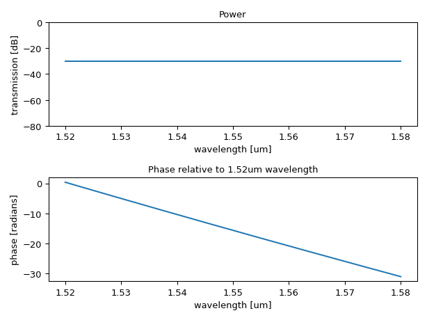
Examples

import numpy as np
import ipkiss3.all as i3
import matplotlib.pyplot as plt

model = i3.cml.WG1(
    center_wavelength=1.55e-6,
    length=100.0 * 1e-6,
    loss=300000.0,
    n_g=2.0,
    n_eff=1.0,
)

wavelengths = np.linspace(1.52, 1.58, 201)
S = i3.circuit_sim.test_circuitmodel(model, wavelengths)

plt.subplot(211)
transmission = 10 * np.log10(np.abs(S["out", "in"]) ** 2)
phase = np.unwrap(np.angle(S["out", "in"]))
plt.plot(wavelengths, transmission)
plt.xlabel("wavelength [um]")
plt.ylabel("transmission [dB]")
plt.ylim([-80, 0])
plt.title("Power")
plt.subplot(212)
plt.plot(wavelengths, phase)
plt.xlabel("wavelength [um]")
plt.ylabel("phase [radians]")
plt.title("Phase relative to 1.52um wavelength")
plt.tight_layout()
plt.show()